The overwhelming scientific consensus is that gases produced by human activity are affecting the global climate. But even if you don’t believe the current warming of the global climate is caused by humans, it’s only common sense that cutting back on human production of heat-trapping gases may help reverse the disturbing recent upward trend in global temperatures.

While politicians attempt to change reality by voting on facts, scientists like me will move forward as best we can to find solutions to the overwhelming problem of climate change.

Agriculture is an often overlooked source of human-produced greenhouse gases. Currently responsible for 10%-12% of global anthropogenic greenhouse gas emissions, it’s a realm ripe for an emissions reduction overhaul. But with the rising global human population, how can farmers increase food production to meet demands while simultaneously cutting back on greenhouse gas emissions? Current research targets ways to mitigate greenhouse gas production while maintaining agricultural productivity, via strategies such as changing how plants are left on fields in the fall, tweaking how much and when fertilizers are added to fields, and adjusting what we feed livestock.

The insulators at issue

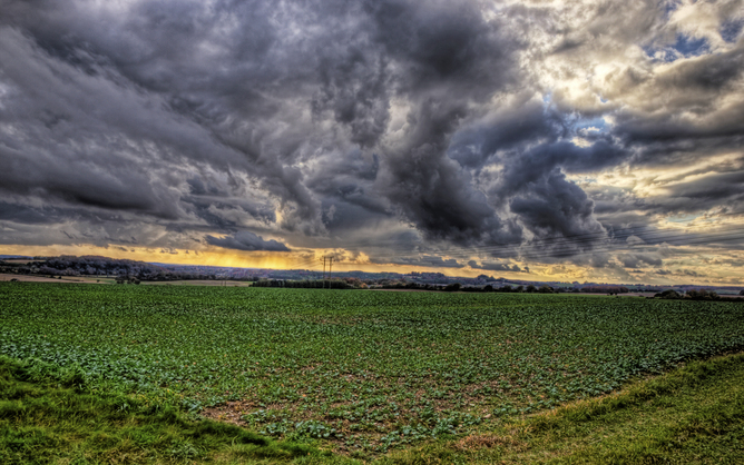
Greenhouse gases absorb infrared radiation – that is, heat. Once in the Earth’s atmosphere, they act as an insulating blanket, trapping the sun’s warmth. Carbon dioxide, the most famous greenhouse gas, is what you exhale with every breath. The main human activity that produces CO2 is the burning of fossil fuels.

Methane and nitrous oxide are also greenhouse gases, and both are produced on farms. Methane comes mainly from rice paddies, manure stockpiles and ruminant animals, such as cattle. Nitrous oxide traces back to nitrogen-containing fertilizers (including manure, commonly the fertilizer of choice for organic farms) added to soils. These gases are of particular concern since they have a greater heat-trapping ability than CO2, meaning that increasing levels of nitrous oxide and methane gases have a greater effect on atmospheric temperature.

Water vapor in the air can also trap heat and so act as a greenhouse gas. Water vapor levels depend on atmospheric temperature, which is in turn affected by levels of heat-trapping gases in the air. By reducing levels of other greenhouse gases in the air, we’ll also reduce the amount of heat-trapping water vapor produced via evaporation of surface water. This has implications for farms that use irrigation.

The natural nitrogen cycle on the farm

All plants need nitrogen, but the form that makes up the majority of the air isn’t readily accessible to them. They depend on the Earth’s nitrogen cycle to convert it to a usable form for them.

Providing nitrogen for their crops is one of the main reasons farmers apply fertilizer, whether organic or synthetic. A natural biological process called denitrification converts the nitrogen in fertilizer (in the form of nitrate or ammonium) to harmless nitrogen gas (N2, a major component in Earth’s atmosphere).

One of the steps in the process of denitrification is the production of nitrous oxide. To complete the denitrification process, bacteria that occur naturally in the soil convert nitrous oxide to N2. However, not every bacterium in the environment that produces nitrous oxide can also reduce it to N2 gas.

The sum of the activity of all denitrifying bacteria in the soil, along with soil chemistry and climatic factors, will affect the relative rates of nitrous oxide consumption or production by a patch of soil. When the amount of fertilizer added to a soil is more than can be taken up and used by plants, bursts of nitrous oxide are often produced. In climates where the ground freezes in winter, spring thaw is often accompanied by bursts of nitrous oxide production as well. These nitrous oxide bursts are an issue for the warming planet.

Methane manufacture

In nature, microorganisms known as methanogens convert simple forms of carbon to methane (CH4). Methane production, or methanogenesis, happens in the absence of oxygen. So waterlogged soils (such as bogs or rice paddies) tend to produce more methane, as do methanogens that live in the rumen (stomach) of ruminant animals, such as cows and sheep.

How to reduce greenhouse gases from farms

There are a number of ways to reduce greenhouse gas emissions from farms, but none is completely simple – the microbial ecosystems in soils and livestock rumens are complex environments, and the tools to study them thoroughly have only really been around for a few decades. But research is under way to tackle greenhouse gas emissions from agriculture, and it’s already clear there are several paths that can help.

We know that, in climates where the ground freezes, overwintering plants on the soil (that is, leaving plants intact on the soil surface after harvest instead of plowing them in or removing them in the fall) can help reduce nitrous oxide emissions. One theory to explain this effect is that the composition and activity of bacterial communities in the soil that produce nitrous oxide gas, or transform these into N2, are affected by soil temperature and nutrients added to the soil. The insulating effect of leaving the plants on the ground surface will affect soil temperature. And the plants contribute nutrients that are added to the soil as they slowly decay during periods above freezing. It’s a complicated system, to be certain, and work into this subject is ongoing.

We also know that limiting inputs of nitrogen to just the amount likely to be usable by plants can reduce emissions. This is easy in principle, of course, but actually guessing how much nitrogen a field full of plants needs to grow well and then supplying just enough to ensure good yields is in practice very difficult. Too little nitrogen and your plants may not grow as well as they should.

Low-input agriculture aims to reduce levels of applied products, including fertilizers, to fields. Along with best management practices, it should help reduce both greenhouse gas production and the environmental impact of farming.

Giving livestock different kinds of food can alter methane emissions from ruminant animals. For example, a greater amount of lipid (fat) in the diet can reduce emissions, but adding too much causes side effects for the animals’ ability to digest other nutrients. Adding nitrate can also reduce methane emissions, but too much nitrate is toxic. Researchers are currently working on modifying the composition of microorganism populations in the rumen to reduce methanogenesis – and thus emissions.

Additionally, it may be possible to add bacteria to soils or to manure digesters to reduce production of nitrous oxide, since certain denitrifying bacteria added to manured soil were able to cut nitrous oxide emissions in a recent study. The bacteria used in this study were naturally occurring organisms isolated from Japanese soils, and similar bacteria are found in soils all around the world.

One of the goals of the lab I work in is to find out how different agricultural management strategies affect the naturally occurring bacteria in the soil, and how these changes relate to levels of nitrous oxide that the soil produces. It may be that, in the future, farmers will use mixtures of bacteria to both promote plant growth and health and mitigate nitrous oxide emissions from the soils on their farms.

Let’s stop waiting

The world is a complicated place – the many different processes that make up global carbon and nitrogen cycles interact in complex ways that we’re still studying. In addition to other solutions engineers have devised that should help reduce emissions, we need to continue working on the agricultural piece of this puzzle.

Elizabeth Bent is Research Associate in Microbiology at University of Guelph.

This article was originally published on The Conversation.
Read the original article.

South Africa’s Karoo region has been in the headlines in recent years because of the prospect of a controversial fracking programme to exploit its potential shale gas resources. But, to palaeontologists, the Karoo Supergroup’s rocks hold the key to understanding the early evolutionary history of the major groups of land vertebrates – including tortoises, mammals and dinosaurs.

More than 200 million years ago, South Africa formed part of the southern hinterland of Pangaea, the great single supercontinent, which was inhabited by a diverse flora and fauna.

In only a few places, where conditions were conducive to their fossilisation, can palaeontologists catch a glimpse of these ancient ecosystems. The Karoo is one such place.

Why it’s such a special place

About 265 million years ago, the Beaufort Group of rocks within the Karoo sequence was beginning to be deposited by rivers draining into the shrinking inland Ecca Sea. As these rivers filled the basin with sediment they entombed the remains of land animals that lived around them. The youngest Beaufort rocks are around 240 million years old.

Today, more than 30,000 fossils of vertebrate animals from the Beaufort reside in museum collections across the world. The Beaufort was followed by the Molteno and Elliot formations. The Elliot formation is made up of a succession of red rocks that records some of the earliest dinosaur communities.

The area plays a crucial role in revealing the distant origin of mammals, tortoises and dinosaurs. It also covers two great extinction events, the end-Permian (252 million years ago) and the end-Triassic (200 million years ago).

Because of its continuity of deposition, the Karoo provides not only a historical record of biological change over this period of Earth’s history, but also a means to test theories of evolutionary processes over long periods of time.

The 400,000 sq km area is internationally noted for its record of fossil therapsid “mammal-like” reptiles. These chart anatomical changes on the path to mammals from their early tetrapod forebears.

The Beaufort Group has also yielded the oldest recorded fossil ancestor of living turtles and tortoises – the small, lizard-like Eunotosaurus. The younger Elliot Formation preserves a record of early dinosaurs that could help palaeontologists understand the rise of the giant sauropod dinosaurs of the Jurassic Period.

Physiology and behaviour

Many studies are still being done on the identification of new species from the Karoo. But a lot of current research is also focused on the relationship between the extinct animals and their environments.

The story of the therapsid’s burrow is a good example of how insights are being gained on the behaviour of prehistoric animals. Roger Smith was the first palaeontologist to recognise therapsid vertebrate burrows in the Karoo. He described helical burrows, which he attributed to a small species of dicynodont (two-dog tooth) therapsid called Diictodon. In the fossil record, burrows are preserved not as hollows, but as the plug of sediment that filled them.

X-ray tomography at a facility in France was recently used to scan one of these burrows. This showed that it was home not only to its maker – the meerkat-sized therapsid Thrinaxodon – but also to the early amphibian Broomistega. Further research revealed that the Thrinaxodon was probably hibernating and this is the reason why it tolerated the intruding amphibian which was using the burrow to convalesce while suffering from broken ribs.

Studying how fossil bones are preserved (taphonomy) can provide similarly rich insights. For example, it has been suggested that changes in preservation style between skeletons in the latest Permian Period (about 253 million years ago) to those in the earliest Triassic Period (about 252 million years ago) can be attributed to changes in climate. The region developed from being seasonally dry floodplains with high water tables to predominantly dry floodplains.

Because of the abundance of fossil tetrapods in the rocks of the Karoo Supergroup, they have been used to divide the rock succession into fossil zones, called biozones. This has enabled the biozones to be correlated with equivalent sequences elsewhere in the world and forms the basis of reconstructing global patterns of diversity.

Understanding the sequence of events is crucial for testing hypotheses of evolutionary processes. It is an area of research being pursued for both the Permian and Triassic periods.

The big wipe-outs

The end-Permian mass extinction, the greatest, was responsible for the elimination of 90% of species living in the sea and 70% of species living on land. Roger Smith’s work on Karoo fossil vertebrates shows this extinction to have lasted approximately 300,000 years, terminating at the Permian-Triassic boundary 252 million years ago. It was followed by a lesser extinction pulse approximately 160,000 years later in the Early Triassic.

Our current work is focusing on the more obscure Guadalupian extinction which occurred eight million to ten million years before the end-Permian. This is recognised from marine sequences. For the first, time empirical evidence for this event on land is being discovered from the Karoo fossil record.

What’s next?

These are exciting times for palaeontologists. Technological and scientific developments have opened up new vistas for their work.

A comprehensive database of all the Karoo fossil vertebrate collections in South Africa has been built. This is the first database of Permian-Jurassic continental vertebrates. It is available to scientists globally, an invaluable tool for biogeographic and biostratigraphic studies.

Better dating techniques are opening up the possibility of working out rates of evolution in fossil tetrapod lineages. High-resolution scanning techniques are also enabling palaeoscientists to explore areas which were previously inaccessible, or at least not without damaging the fossils.

There are a myriad questions that remain unanswered. Were the early mammal ancestors of the Karoo warm-blooded? What can the Karoo tell us about the reaction of terrestrial ecosystems to mass extinction events? How can the Karoo’s shifting ecological make-up shine a light on evolutionary tempo? These are questions we can now attempt to answer.

Bruce Rubidge is Director, Centre of Excellence in Palaeosciences at University of the Witwatersrand.
Mike Day is Postdoctoral Fellow, Evolutionary Studies Institute at University of the Witwatersrand.

This article was originally published on The Conversation.
Read the original article.

It’s very hard to overstate how important the US power grid is to American society and its economy. Every critical infrastructure, from communications to water, is built on it and every important business function from banking to milking cows is completely dependent on it.

And the dependence on the grid continues to grow as more machines, including equipment on the power grid, get connected to the Internet. A report last year prepared for the President and Congress emphasized the vulnerability of the grid to a long-term power outage, saying “For those who would seek to do our Nation significant physical, economic, and psychological harm, the electrical grid is an obvious target.”

The damage to modern society from an extended power outage can be dramatic, as millions of people found in the wake of Hurricane Sandy in 2012. The Department of Energy earlier this year said cybersecurity was one of the top challenges facing the power grid, which is exacerbated by the interdependence between the grid and water, telecommunications, transportation, and emergency response systems.

So what are modern grid-dependent societies up against? Can power grids survive a major attack? What are the biggest threats today?

The grid’s vulnerability to nature and physical damage by man, including a sniper attack in a California substation in 2013, has been repeatedly demonstrated. But it’s the threat of cyberattack that keeps many of the most serious people up at night, including the US Department of Defense.

Why the grid so vulnerable to cyberattack

Grid operation depends on control systems – called Supervisory Control And Data Acquisition (SCADA) – that monitor and control the physical infrastructure. At the heart of these SCADA systems are specialized computers known as programmable logic controllers (PLCs). Initially developed by the automobile industry, PLCs are now ubiquitous in manufacturing, the power grid and other areas of critical infrastructure, as well as various areas of technology, especially where systems are automated and remotely controlled.

One of the most well-known industrial cyberattacks involved these PLCs: the attack, discovered in 2010, on the centrifuges the Iranians were using to enrich uranium. The Stuxnet computer worm, a type of malware categorized as an Advanced Persistent Threat (APT), targeted the Siemens SIMATIC WinCC SCADA system.

Stuxnet was able to take over the PLCs controlling the centrifuges, reprogramming them in order to speed up the centrifuges, leading to the destruction of many, and yet displaying a normal operating speed in order to trick the centrifuge operators. So these new forms of malware can not only shut things down but can alter their function and permanently damage industrial equipment. This was also demonstrated at the now famous Aurora experiment at Idaho National Lab in 2007.

Securely upgrading PLC software and securely reprogramming PLCs has long been of concern to PLC manufacturers, which have to contend with malware and other efforts to defeat encrypted networks.

The oft-cited solution of an air-gap between critical systems, or physically isolating a secure network from the internet, was precisely what the Stuxnet worm was designed to defeat. The worm was specifically created to hunt for predetermined network pathways, such as someone using a thumb drive, that would allow the malware to move from an internet-connected system to the critical system on the other side of the air-gap.

Internet of many things

The growth of smart grid – the idea of overlaying computing and communications to the power grid – has created many more access points for penetrating into the grid computer systems. Currently knowing the provenance of data from smart grid devices is limiting what is known about who is really sending the data and whether that data is legitimate or an attempted attack.
This concern is growing even faster with the Internet of Things (IoT), because there are many different types of sensors proliferating in unimaginable numbers. How do you know when the message from a sensor is legitimate or part of a coordinated attack? A system attack could be disguised as something as simple as a large number of apparent customers lowering their thermostat settings in a short period on a peak hot day.

Defending the power grid as a whole is challenging from an organizational point of view. There are about 3,200 utilities, all of which operate a portion of the electricity grid, but most of these individual networks are interconnected.

The US Government has set up numerous efforts to help protect the US from cyberattacks. With regard to the grid specifically, there is the Department of Energy’s Cybersecurity Risk Information Sharing Program (CRISP) and the Department of Homeland Security’s National Cybersecurity and Communications Integration Center (NCCIC) programs in which utilities voluntarily share information that allows patterns and methods of potential attackers to be identified and securely shared.

On the technology side, the National Institutes for Standards and Technology (NIST) and IEEE are working on smart grid and other new technology standards that have a strong focus on security. Various government agencies also sponsor research into understanding the attack modes of malware and better ways to protect systems.

But the gravity of the situation really comes to the forefront when you realize that the Department of Defense has stood up a new command to address cyberthreats, the United States Cyber Command (USCYBERCOM). Now in addition to land, sea, air, and space, there is a fifth command: cyber.

The latest version of The Department of Defense’s Cyber Strategy has as its third strategic goal, “Be prepared to defend the US homeland and US vital interests from disruptive or destructive cyberattacks of significant consequence.”

There is already a well-established theater of operations where significant, destructive cyberattacks against SCADA systems have taken place.

In a 2012 report, the National Academy of Sciences called for more research to make the grid more resilient to attack and for utilities to modernize their systems to make them safer. Indeed, as society becomes increasingly reliant on the power grid and an array of devices are connected to the internet, security and protection must be a high priority.

Michael McElfresh is Adjunct Professor of Electrical Engineering at Santa Clara University.

This article was originally published on The Conversation.
Read the original article.

This article is part of The Conversation’s series this month on hurricanes. You can read the rest of the series here.

In the US, the 2015 hurricane season begins against a backdrop of other recent extreme weather news. Texas floods and Midwest tornadoes remind us of what water and wind can do. We can take comfort from considerable improvement in hurricane forecast accuracy in recent years. But when a hurricane is gathering strength offshore, people in its possible line of fire still need to decide whether or not to evacuate to safer ground.

As a social scientist, I’ve been interested in what goes into the choice whether to stay or to go, and whether people will have time to leave if that’s what they choose to do. It’s a complex decision that can be a matter of life and death. Why do some people evacuate and some do not? We’re finding that timing can have a lot to do with it.

Getting out of a storm’s path saves lives

Consider the comparison of lives lost due to Hurricanes Katrina and Sandy. Forty-one people drowned from Sandy’s storm surge and 31 others died from falling trees and other causes. Katrina killed more than 1,800 people. Over half of the Mississippi evacuation zone residents heeded the call and left ahead of Katrina. That compares with about 30% for Sandy, according to my own survey research.

Comparing populations between coastal Mississippi and New Jersey/New York, a storm like Katrina could have translated to many thousands of deaths if it had hit the New York metropolitan area.

It wasn’t evacuation that made a difference in the number of lives saved. The sobering conclusion is that it was just luck that Sandy, hitting a much more populous area, had weaker winds blowing over people trying to evacuate the day the storm arrived. But the next storm through could have much more intense winds. That potential scenario makes it crucial to examine why there was such a low evacuation rate for Sandy – and how to make sure a future situation would have a higher one.

What goes into the decision to leave

Most behavioral studies show hurricane evacuation rates can be explained by a number of factors, including media communication of forecast risk, physical risk at a person’s location, demographics (for instance, people with young children are more likely to evacuate, while the elderly often find it harder to do so), and availability of transportation resources, as well as a place to go.

However these factors never explain more than half the variance in evacuation. The rest is the hard part, what psychologist Paul Slovic calls “intuitive risk judgments.” Certainly there are some people who believe they’ll be safe no matter what. But most people routinely do a good job of deciding to do things like buying insurance against big dangers that are not very likely to happen.

The problem for the public in hurricane evacuation is not the probability part; it’s the danger part, whether storm surge could actually happen to me and result in my death or loss of livelihood. It’s vital that everyone, politicians as well as the public, is educated about how storm surge works and the risks affiliated with it. When people aren’t sure but get scared they will go ahead and evacuate, even when the result is unnecessary traffic gridlock, as happened in hurricanes Floyd and Rita.

So the problem for forecasters, media and authorities is threefold: make sure the people at risk know they are, make sure people who can safely stay home know that, and get those two groups of people informed far enough ahead of time that they can know what to do when evacuation orders come down. To accomplish these goals, precise locational information on surge risk is needed – such as will be provided by the new Potential Storm Surge Flooding Map developed by the National Hurricane Center.

This kind of map can be made available up to 36 hours ahead of hurricane landfall once surge modelers know what the characteristics of the storm will be as it approaches land. Before that, an accurate forecast is not possible because location and height of storm surge is heavily dependent on the hurricane’s track, size and strength, as well as the configuration of near-shore bays and other water bodies, and underwater terrain where it hits.

People need time

Few studies have looked at what happens next, once people realize they need to evacuate. Timing appears to be a crucial factor.

Studies indicate that authorities need to allow a full 24 hours after definitive evacuation orders for people to get ready and actually leave. Preparing to go, coordinating work and family members, and organizing transportation can take a full day. And after that, evacuees may need 10 hours of daylight to travel before hurricane force winds arrive.

Hurricane Evacuation Studies are done by the US Army Corps of Engineers. These incorporate behavioral studies and traffic modeling to predict clearance times to get everyone out of evacuation zones, assuming good compliance with evacuation orders. Clearance times for the Miami area, for instance, run 20 to 30 hours, depending on the size of storm forecast.

As noted above, this 24+10 hour time frame is approximately how far out hurricane forecasters can accurately predict where storm surge impact is likely to be. So in this case the limits of our forecasting technology fit with the limits of human preparation. The trouble comes in if the 10-hour period for travel turns out to be at night. Postponing departure until morning, which is human nature, means evacuating and traveling through tropical storm force or higher winds. Hurricanes Ivan and Sandy both fit this scenario, with people evacuating through tropical storm force winds. Hurricanes Katrina and Andrew did not, because their time frames were 12 hours different, allowing people to travel during daylight before the storms arrived in the early hours of the morning.

The time potentially needed for evacuation thus makes it essential that the public knows what the worst case for storm surge could be for them and is alerted to the need to plan for a possible evacuation order. The National Hurricane Center has maps of worst-case storm surge scenarios for any configuration of possible hurricanes along the US coastline. Emergency managers use these routinely, but media and authorities need to communicate to the public where people must be alert to risk and also where people can know they will not have to evacuate in any hurricane scenario.

What we need to hear, and when

Emergency managers are charged with ensuring the safety of the population. “Prepare for the worst” is probably a good philosophy in most circumstances, but not in the case of evacuation for a hurricane many days away, when the cost of mobilizing is high and the probability of it being needed is very low. The government and media also grapple with not wanting to be unnecessarily alarmist. The correct philosophy is “know what the worst case could be and be prepared to face it if it comes to pass.”

When an evacuation order is issued, it’s usually in a very compressed time frame – but that’s ok as long as people are prepared. If people plan three to five days ahead, knowing that there is a small but real chance they will be asked to evacuate and a small but real chance of death if they do not, they can be ready when the definitive order comes in.

Hugh Gladwin is Associate Professor of Global and Sociocultural Studies at Florida International University.

This article was originally published on The Conversation.
Read the original article.

Texas has suffered damaging floods and record rainfall in May after years of punishing drought. We asked John Nielsen-Gammon, professor of atmospheric sciences at Texas A&M University and Texas state climatologist, to discuss how climate scientists – and the general public – can sort out when extreme weather events can and can’t be connected to the effects of climate change.

What’s causing the heavy rains behind the dramatic flooding in Texas last week?

We have had a moderate El Niño in the tropical Pacific develop this spring, and it is unusually strong for this time of year. Whenever you have an El Niño, it increases the temperature difference from the tropics to the higher latitudes, and that intensifies the jet stream and pulls it a little closer to the tropics. And since Texas is 25 to 37 degrees north, that can make a difference in what kind of weather we get.

Usually, that effect tends to tail off toward the end of March because the jet stream moves farther north. But we’ve seen an unusually active subtropical jet stream this month, and it has the hallmarks of being caused by what’s going on in the tropical Pacific. So that’s a necessary aspect of what we’re seeing, because it brings cool air aloft on top of the warm moisture we’re getting from the Atlantic. It also helps produce upward motion, which also destabilizes the atmosphere and triggers convection.

Is there a climate change signature with the intense flooding in Texas?

There are several ways of looking at it, and it partly depends on what aspect of the event you’re concerned about. For example, the biggest problem in terms of public safety with the rain is localized heavy rain and flooding events. In Texas, they do happen fairly often when all moisture in the atmosphere is converted to rainfall in a small area.

Thermodynamically, there’s a limit to how much water vapor can be carried by the air; it depends on the temperature. And the ocean temperatures have increased overall, which means the carrying capacity of moisture in the air has also increased. So the maximum amount of rainfall you can get from one particular rainfall event has also increased.

Studies have shown the odds of very intense rainfall in this part of the country have gone up substantially over last century. The cause and effect with climate change and surface temperature is fairly direct. There’s definitely a connection there.

In terms of the overall weather pattern, we do not know if El Niño will be more frequent or less frequent because of climate change. Overall, we can’t say that the weather patterns that led to the wet conditions this month have had any relationship to climate change that we know of.

What do climate change models say about drought?

It depends on how you measure drought. The biggest factor driving drought in Texas and the Great Plains in general is rising temperatures. It’s not clear yet whether the rising temperatures are going to outpace the increase in rainfall that’s been observed to lead to more or less drought overall.

We certainly know climate change is going to make temperatures warmer, make evaporation more intense and increase water demand for plants and agriculture, so it will make that aspect of drought worse. But it remains to be seen whether droughts overall will become worse, because that depends on rainfall. Since models are generally projecting a rainfall decrease, model-based analyses show some pretty nasty increases in drought intensity in the area.

What does it mean to have more extreme weather events from climate change?

I think people take it ordinarily to mean that weather will be more variable. And that’s not necessarily the case. Indeed, most who have looked at changes in temperature have found no increases in variability except maybe in the Arctic, where there used to be more sea ice but there isn’t any more, which does lead to be more variability there. But not for most of the rest of us.

But if you think about extremes in terms of comparing to historic norms, as we get warmer we’ll see more record high temperature events and fewer record low temperature events. And it’s asymmetric, because if you imagine the low record temperatures events, you go from very few of them to none of them, and high temperature events go from very few of them to a whole lot of them, depending on how hot it gets.

So you do end up getting more extremes, even if the range between how hot it gets and how cold it gets doesn’t change, because you’re measuring extremes relative to a different climate in the past.

Also, extremes can be extremely unusual, or they can be extremely damaging – they’re really two separate concepts. Extremely damaging events are droughts, floods, hurricanes and tornadoes. And for those, you have to break it out event by event and phenomenon by phenomenon and consider each in turn.

In the case of heavy local rainfall, trends have been detected and the models predict an increasing trend, so that’s a pretty solid one. With hurricanes, no trend has been detected, but models predict an increasing trend and we understand why. We’re not as confident in increased intensity of hurricanes, but still the evidence points in that direction. The trouble with detecting a trend is that rare events happen erratically, so it’s hard to tell if you really have a trend or it’s just randomness going on. On the other hand, there could be a trend but the randomness can make it hard to tell for sure.

If climate scientists don’t have a long record to work with, how can they predict weather events and their link to climate change?

If you don’t have the historic trend to rely upon, you can do experiments with the climate models. They aren’t exact replicas of the Earth, but they are simulations of a planet very much like our own. You can plug in different ocean temperature patterns and different conditions to see what results it has on weather, and get cause-and-effect relationships that way. Running the model for really long periods of time can detect trends that aren’t detectable just with historic records.

Given the uncertainties in this process, what are some of the challenges in communicating the role of climate change in weather to the public and policymakers?

One challenge is that usually it’s an ill-posed question. People care about individual events, but all you can do is compare actual events to hypothetical events that might have happened otherwise. So it’s not a real comparison; it’s a hypothetical comparison.

What we can do is to look at changes in the odds of things happening. But all you can say is events meet a certain definition of being this much more likely or less likely. So it gets away from talking about specific events to a set of events.

Another challenge is that the public has gotten the impression, because it’s been repeated, that climate change is going to be causing more extremes. But you really can’t generalize; you have to talk about which types of extremes and where.

For example, we do expect climate change to cause more flood and rain events. We also expect more droughts. However, the area of the globe that would experience both of those simultaneously is probably less than half the Earth’s surface.

In others words, some places will get enough rainfall to reduce the amount of drought. Some places will get less rainfall, so they’ll have fewer floods. It’s going to be the unlucky few that will get both of them, but people perceive that it’s supposed to happen to everybody.

What is the ultimate goal of studying the links between extreme weather and climate change?

The aspect of event attribution is a still an immature science. People are working on it because the public seems to care so much about it. But it doesn’t really matter for scientific or planning purposes how specific events have been affected by climate change. What matters is the likelihood of future events being affected, because those are the ones you can plan for.

People want to sway public opinion about that urgency of climate change so past and current events get all the attention. As long as scientists don’t overstate the results, it’s OK to talk about this. But it’s more useful for making people aware of climate change than it is for planning or making society more resilient to future impacts.

John Nielsen-Gammon is Regents Professor of Climatology at Texas A&M University .

This article was originally published on The Conversation.
Read the original article.

This article is part of The Conversation’s series this month on hurricanes. You can read the rest of the series here.

Every year, typhoons over the western North Pacific – the equivalent to hurricanes in the North Atlantic – cause considerable damage in East and Southeast Asia.

Super Typhoon Haiyan of 2013, one of the strongest ocean storms ever recorded, devastated large portions of the Philippines and killed at least 6,300 people. It set records for the strongest storm at landfall and for the highest sustained wind speed over one minute, hitting 315 kilometers (194 miles) per hour when it reached the province of Eastern Samar.

The situation may get even worse.

Our new study of what controls the peak intensity of typhoons, published in the journal Science Advances, suggests that under climate change, storms like Haiyan could get even stronger and more common by the end of this century.

Disentangling factors in typhoon peak intensity

The lifetime peak intensity of a typhoon is the maximum intensity the storm reaches during its entire lifetime. It results from an accumulation of intensification, which is equivalent to speed being an accumulation of acceleration.

To better understand the variability and changes in typhoon peak intensity, we employed a novel approach by decomposing the peak intensity (akin to speed) into two components: intensification rate (akin to acceleration) and intensification duration (akin to time). These two components vary independently from each other from one year to another. We then separately explored the climate conditions that were most strongly associated with the year-to-year variations in these two components.

We examined various atmospheric and oceanic variables that might influence the rate of cyclone intensification.

We looked at atmospheric pressure, vertical wind shear, or the change in wind speed in one direction, and vorticity, or the spin of the atmosphere. Surprisingly, we found that compared to those factors, ocean temperature most strongly correlated to the rate of cyclone intensification.

Specifically, how strongly and quickly a cyclone can grow depends on two oceanic factors: pre-storm sea surface temperature and the difference in temperature between the surface and subsurface.

A warmer sea surface generally provides more energy for storm development and thus favors higher intensification rates.

A large change in temperature from the surface to subsurface (ie, cooling with depth), however, can disrupt this flow of energy. That’s because strong winds drive turbulence in the upper ocean, which brings cold water up from below and cools the sea surface. Therefore, a smaller difference between surface and subsurface ocean temperature favors higher intensification rates.

On the other hand, the variations in the duration of typhoon intensification can be connected to sea surface temperatures associated with the naturally occurring phenomena known as El Nino-Southern Oscillation/Pacific Decadal Oscillation (ENSO/PDO). This is because in a positive phase of ENSO/PDO, warmer-than-normal sea surface temperatures over the central equatorial Pacific produce favorable atmospheric conditions for cyclone genesis near the equator and dateline. This allows developing typhoons to grow for a longer period of time over the warm water before reaching land or cold water.

In sum, our analyses reveal that the upper-ocean temperatures over the low-latitude western North Pacific influence typhoon intensification rates, and that sea surface temperatures over the central equatorial Pacific influence typhoon intensification duration.

We then quantified the relationships between typhoon peak intensity and these identified climatic factors – that is, local upper ocean temperatures and ENSO/PDO indices.

We concluded that the strong rise in typhoon peak intensity over the past 35 years or so (about five meters per second; equivalent to half a category in typhoon strength) can be mostly attributed to unusual local upper-ocean warming rates.

Projecting typhoon peak intensity in a warming climate

We analyzed the ocean temperature changes simulated by models from the fifth phase of the Coupled Model Intercomparison Project (CMIP5), a model for studying interactions between ocean and the atmosphere.

We found that by year 2100, the temperature of the upper ocean will be more than 1.6 degrees Celsius higher than the baseline average of the 50-year period from 1955-2005 even under a moderate future scenario of greenhouse gas emissions.

The continued ocean warming provides more “fuel” for storm intensification. Using the statistical relationships built from observations, we projected that the intensity of typhoons in the western North Pacific will increase as much as 14% – nearly the equivalent to an increase of one category – by century’s end.

Wei Mei is Postdoctoral Scholar at Scripps Institution of Oceanography at University of California, San Diego.

This article was originally published on The Conversation.
Read the original article.