Category Archives: Environment

Tipping point: how we predict when Antarctica’s melting ice sheets will flood the seas


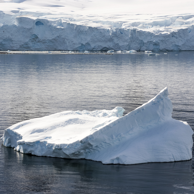
Antarctica is already feeling the heat of climate change, with rapid melting and retreat of glaciers over recent decades.

Ice mass loss from Antarctica and Greenland contributes about 20% to the current rate of global sea level rise. This ice loss is projected to increase over the coming century.

A recent article on The Conversation raised the concept of “climate tipping points”: thresholds in the climate system that, once breached, lead to substantial and irreversible change.

Such a climate tipping point may occur as a result of the increasingly rapid decline of the Antarctic ice sheets, leading to a rapid rise in sea levels. But what is this threshold? And when will we reach it?

What does the tipping point look like?

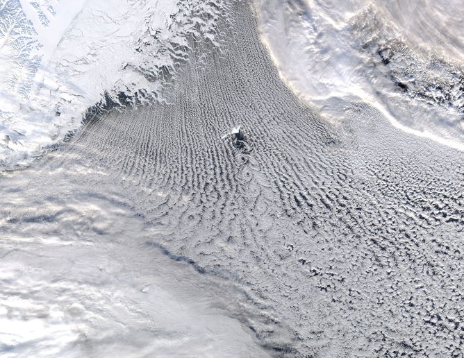
The Antarctic ice sheet is a large mass of ice, up to 4 km thick in some places, and is grounded on bedrock. Ice generally flows from the interior of the continent towards the margins, speeding up as it goes.

Where the ice sheet meets the ocean, large sections of connected ice – ice shelves – begin to float. These eventually melt from the base or calve off as icebergs. The whole sheet is replenished by accumulating snowfall.

Emperor penguins at sunrise.
David Gwyther

Floating ice shelves act like a cork in a wine bottle, slowing down the ice sheet as it flows towards the oceans. If ice shelves are removed from the system, the ice sheet will rapidly accelerate towards the ocean, bringing about further ice mass loss.

A tipping point occurs if too much of the ice shelf is lost. In some glaciers, this may spark irreversible retreat.

Where is the tipping point?

One way to identify a tipping point involves figuring out how much shelf ice Antarctica can lose, and from where, without changing the overall ice flow substantially.

A recent study found that 13.4% of Antarctic shelf ice – distributed regionally across the continent – does not play an active role in ice flow. But if this “safety band” were removed, it would result in significant acceleration of the ice sheet.

The Totten Glacier calving front.
Esmee van Wijk/CSIRO

Antarctic ice shelves have been thinning at an overall rate of about 300 cubic km per year between 2003 and 2012 and are projected to thin even further over the 21st century. This thinning will move Antarctic ice shelves towards a tipping point, where irreversible collapse of the ice shelf and increase in sea levels may follow.

How do we predict when will it happen?

Some areas of West Antarctica may be already close to the tipping point. For example, ice shelves along the coast of the Amundsen and Bellingshausen Seas are the most rapidly thinning and have the smallest “safety bands” of all Antarctic ice shelves.

To predict when the “safety band” of ice might be lost, we need to project changes into the future. This requires better understanding of processes that remove ice from the ice sheet, such as melting at the base of ice shelves and iceberg calving.

Melting beneath ice shelves is the main source of Antarctic ice loss. It is driven by contact between warmer sea waters and the underside of ice shelves.

To figure out how much ice will be lost in the future requires knowledge of how quickly the oceans are warming, where these warmer waters will flow, and the role of the atmosphere in modulating these interactions. That’s a complex task that requires computer modelling.

Predicting how quickly ice shelves break up and form icebergs is less well understood and is currently one of the biggest uncertainties in future Antarctic mass loss. Much of the ice lost when icebergs calve occurs in the sporadic release of extremely large icebergs, which can be tens or even hundreds of kilometres across.

It is difficult to predict precisely when and how often large icebergs will break off. Models that can reproduce this behaviour are still being developed.

Scientists are actively researching these areas by developing models of ice sheets and oceans, as well as studying the processes that drive mass loss from Antarctica. These investigations need to combine long-term observations with models: model simulations can then be evaluated and improved, making the science stronger.

The link between ice sheets, oceans, sea ice and atmosphere is one of the least understood, but most important factors in Antarctica’s tipping point. Understanding it better will help us project how much sea levels will rise, and ultimately how we can adapt.

The Conversation

Felicity Graham, Ice Sheet Modeller, Antarctic Gateway Partnership, University of Tasmania; David Gwyther, Antarctic Coastal Ocean Modeller, University of Tasmania; Lenneke Jong, Cryosphere System Modeller, Antarctic Gateway Partnership & Antarctic Climate and Ecosystems CRC, University of Tasmania, and Sue Cook, Ice Shelf Glaciologist, Antarctic Climate and Ecosystems CRC, University of Tasmania

This article was originally published on The Conversation. Read the original article.

Why it makes little sense to regulate rainwater barrels in the dry western U.S.


Many of us never think about who gets to use the drops of rain that fall from the sky. But it’s an increasingly pertinent question as more people look to collect rainwater as a way to conserve water, live off the grid or save money on water bills.

As a result, many states in the arid West are now asking whether rain barrels are allowed under existing law and policy and, in some cases, are setting limits on the practice of rainwater catchment.

Colorado has gone further than any of its neighbors by requiring a permit for any rainwater collection. Meanwhile, Utah put rainwater harvesting rules into effect in 2010 with some restrictions, and Washington legalized rainwater collection in 2009, while leaving the state the “ability to restrict if there are negative effects on instream values or existing water rights.”

Why this worry over rainwater harvesting?

If everyone captures the rain that falls on rooftops and through downspouts of homes, the argument goes, then the water will never reach the rivers and streams. If this happens, existing water users may not be able to access their rights to use the water.

This concern, however, overstates the issue and risks missing more concrete opportunities for water conservation and efficiency. A more effective way to address decreasing water supply would be for states to apply the legal principles prohibiting waste and demanding reasonable water use, which have long been embedded in any right to use water.

U.S. water law, east and west

Both the rainwater collectors and the existing water rights holders, such as irrigators or municipalities with water rights to river flows or groundwater sources, believe they have a fully private interest in any water they use.

Throughout the United States, however, the law recognizes the public nature of water. Under the public trust doctrine, each state holds title to the water within the state in trust for the people of the state.

Given the competing demands for water use, principles of U.S. law seek to balance these competing needs and uses to ensure that the public’s rights to water are protected.

In western states, farm owners often have rights to use water which can often be delivered through irrigation ditches, such as this one in Colorado.
question_everything/flickr, CC BY-NC-ND

In the eastern United States, there is the riparian system that protects reasonable use of water among all landowners along rivers or streams. In the western part of the country, the doctrine of prior appropriation requires a permit to use water based on showing that the water will be put to beneficial use without waste.

The public nature of water ensures that individual private interests never fully control who gets access to water and when, where and how water is used. In fact, when an individual has a right to use water, that right is known as a “usufructory” interest – that is, the right to use the water without owning the water itself.

Granting a usufructory interest – something that doesn’t fully privatize a water right – makes good sense when you think about the nature of water.

Short of putting water in a bottle and selling it by the ounce, water is difficult to possess and reduce to ownership. It is a shared resource that is used over and over again as the molecules of water make their way through the hydrologic system.

Water falls from the sky, runs along the ground and percolates into the groundwater system. It is taken up by plants and trees, consumed by people and animals, and eventually makes its way through one mechanism or another, back into the groundwater or surface water sources, only to flow further down the system to be used again or eventually evaporate back into the atmosphere to start the process all over again.

Private ownership of drops of water presents a complex problem not only as a legal matter, but as an ethical public policy choice as well.

The debate over rainwater collection demonstrates this complexity.

Don’t homeowners in Colorado have the right to collect rain that falls on their rooftop? At the same time, doesn’t a senior water right holder have a right to have the rain enter the stream so that their right can be satisfied?

Our legal system evolved ways to deal with this complex reality, with our state governments empowered to manage this resource among competing interests on behalf of all of us.

In the eastern United States where rainfall is plentiful and competing uses for water are rare, the riparian system allows any landowner adjacent to a water source to use its water. If there is a conflict about the quantity of water available for a certain use, that conflict is resolved by using legal standards to sort through the reasonableness of each individual’s use.

In the western United States, where competition among users has always been more commonplace, each individual state requires a permit for water use. These permits are awarded pursuant to the doctrine of prior appropriation. For example, irrigated agriculture often holds senior water rights (issued under state law) and Indian tribes often hold even more senior rights (based on federal law).

When conflict arises, disputes are resolved using the legal principle of first-in-time, first-in-right that protects the most senior, beneficial, nonwasteful uses of water. Or at least that is the theory.

Water waste and powerful interests

So how does this relate to the regulation of rainwater harvesting?

If the primary concern is that somehow rainwater barrels will limit the amount of water in the system, reduce availability of water and potentially impact existing rights, then there may be better ways to address this concern.

Rather than devoting resources to regulating individual rain barrels – a logistically difficult task – it may make more sense for state water agencies to get serious about enforcing principles of waste.

To enforce waste reduction policies, water resource management agencies in each state would need to set standards on how much water is needed to carry out a particular use. They then would need to measure water use to ensure that individual permit holders are not taking more water than what is necessary to accomplish their purpose.

Many longstanding water users take more water than they need, under the principle of use-it-or-lose-it. In western water law, if you don’t use the water, you risk forfeiting your water right. As a result, many users divert the full quantity of their water right whether that amount is needed or not.

If the states crack down on waste, it will bring this longstanding practice into the spotlight. Existing water users may be faced with calls to increase efficiency and to decrease the rate of diversion.

As droughts become more frequent and demands on water grows, states could do more to reduce waste from big water users.
sunlizard4fun/flickr, CC BY

For decades, there has been a persistent reluctance to address waste because it would involve scrutinizing water use practices among some of the most powerful interests in the state.

But by addressing the thorny problem of waste, state agencies could make more headway in securing reliable water supplies and certainly could have a more significant impact on water supply than regulating rainwater catchment.

In the end, we may face tough public policy choices about whether and how to regulate rainwater catchment. But before we go in this direction, policymakers should take a careful look at whether existing larger-scale water users are complying with longstanding principles of nonwaste and reasonableness embedded in U.S. water law.

The Conversation

Adell Amos, Associate Dean for Academic Affairs, Associate Professor of Environmental and Natural Resources Law, University of Oregon

This article was originally published on The Conversation. Read the original article.

Why legal challenges to the EPA Clean Power Plan will end up at the Supreme Court


Cara Horowitz, University of California, Los Angeles

Even before President Obama announced the Environmental Protection Agency’s (EPA) Clean Power Plan on August 3 to regulate carbon emissions from power plants, there were a number of legal challenges to block the law at its proposal stage – none of them successful. Earlier this year, the DC Circuit Court told opponents, which included a coal company joined by 12 states, that their arguments were premature.

Now that the rules are final, the new court challenges will come fast and heavy. The legal arguments against the plan will be focused on two issues.

The first is based on an unusual legislative drafting inconsistency, whereby the House and Senate versions of the key Clean Air Act provision lead to different conclusions about the EPA’s authority here. In the rush to complete its 1990 amendments to the Clean Air Act, Congress allowed two inconsistent versions of the statute to pass through the conference committee, never to be reconciled. One would allow regulation of carbon dioxide from power plants under the provision being used in the Clean Power Plan; the other arguably would not. No court has ever addressed the question. Call this a drafting-error argument.

More centrally, the Clean Air Act language at issue is inherently ambiguous, as many texts are. It calls for the EPA to set standards for pollution reduction that are based on the “best system of emission reduction” that has been “adequately demonstrated.” Any first-year law student would know to ask: What’s a “system”? How do we know what’s the “best system”? And what level of demonstration is “adequate”?

Counter to conservative thinking

The EPA has taken a broad view of these terms, setting pollution reduction standards that assume states can, and should, do a lot to limit carbon dioxide from fossil fuel–powered plants. That includes things far outside the fenceline of those plants, such as creating incentives to ramp up solar power installations in urban neighborhoods.

To the EPA, “systems” are capacious, and “best” means we shouldn’t think small. Opponents in industry counter that this provision was never about making changes outside the property lines of the regulated emissions sources themselves. To them, the EPA’s stance is an unauthorized reach.

Both the drafting-error argument and the statutory ambiguity argument will come down to how much discretion one thinks the EPA should have to interpret its own legislative mandates.

Will the Supreme Court ultimately decide the EPA Clean Power Plan’s fate?
bootbearwdc/flickr, CC BY

Traditionally, courts have deferred to agencies where they are acting in their areas of delegated power. And there are good reasons for courts to curtail the instinct to second-guess expert agencies when statutes can be interpreted more than one way. But this tradition of deference has run smack into the modern line of conservative thinking that maligns federal bureaucracy.

This case will almost certainly reach the US Supreme Court, given the force and funding of the opposition and the importance of the issue to federal energy policy. If and when it does reach the highest court, it is hard to say whether the EPA’s rule will be seen as an agency power grab, or, alternatively, as a reasonable exercise of authority given mandates that necessarily require interpretation.

The court’s most recent environmental cases suggest that the agency is on a shortening leash. Earlier this year, the Supreme Court ruled that the EPA misinterpreted the Clean Air Act in regulating mercury levels from power plants, by failing to consider costs early enough. The court’s reasoning betrayed an impatience with deferring to the EPA.

For now, we can only wait to see how the legal drama will play out.

The Conversation

Cara Horowitz, Co-Executive Director, Emmett Institute on Climate Change and the Environment, UCLA School of Law, University of California, Los Angeles

This article was originally published on The Conversation. Read the original article.

Legacy of Abandoned Gold Mines Means More Spills


Canary in the Gold King Mine: legacy of abandoned mines means more spills

Ronald R H Cohen, Colorado School of Mines

You are gazing over the clear stream, thinking of fishing the crystal waters in the Rockies. The next morning, you are stunned to see an orange-yellow sludge covering the stream as far as you can see. Is this the Colorado Gold King Mine spill into Cement Creek of August 5, 2015?

No, this describes the Clear Creek, CO spill of April, 2009 from a private mine or it could be the 1975 or 1978 Cement Creek spills from abandoned mines.

Spills of acid mine drainage (AMD) from abandoned mines have been a problem in the US for over 100 years.

How many other mines are leaking or holding millions of gallons of toxic wastewater? And how can we avoid these types of damaging spills in the future?

To the source

AMD, also known as acid-rock drainage (ARD) and mining-influenced water (MIW), results from the exposure of sulfide minerals, particularly pyrite (also known as fool’s gold), to oxygen and water. Then, biological and chemical reactions generate sulfuric acid and mobilize heavy metals associated with the rocks and ore.

Acidic wastewater with heavy metals spills from the opening of the Gold King Mine in photo released by the EPA.
Reuters

AMD wastewater can be characterized by high acidity, elevated heavy metals as well as relatively high concentrations of sulfates and solid particles (suspended solids). Iron that is chemically bound to the solid particles give that orange-yellow color. The old-time miners called it “yellow boy.”

When a mine is dug, eventually water will be encountered. To maintain dry workings, the water is pumped out or a tunnel is dug underneath the work area to drain the water. When the mine ceases operations, the pumps are turned off and the mine begins to fill with water.

Under certain conditions, the water, perhaps contaminated with AMD, will decant or discharge out of the mine workings. The predominant AMD generating source in the Western United States is metal mine workings, whose drainage often contains cadmium, lead, nickel, copper and zinc.

Heavy metals

The Gold King Mine is one of many abandoned mines on the Colorado landscape. The Bureau of Land Management, (BLM) in Colorado maintains an ongoing inventory in the State and in 2008 reported 2,751 known abandoned hard rock mines on public lands. The inventory included 4,670 features of mines, such as draining openings and shafts, and mine waste, that may impact water resources.

The numbers of abandoned mines discovered increases every year, rising from a total of 19,000 abandoned mines in 2008 to over 28,000 in 2011.

In order to determine the behavior and impacts of the spill, it is necessary to know the chemical and physical aspects of the spill, and the characteristics of the receiving waters.

In the case of the Gold King spill on August 5, the Cement Creek has been exposed to input of mine drainage on a continuous basis for 100 years. The Cement Creek feeds into the Animas River which then flows to Durango, CO and down the San Juan River to New Mexico and Utah, and ultimately into Lake Powell.

Even before measurements were released to the public, we can assume that the water in the spill would be acidic, there would be solid particles containing high levels of iron and some other metals, and that there would be concentrations of metals dissolved in the water above stream standards. Metals become more soluble in the water as the pH decreases and acidity increases.

The spill was estimated to be three million gallons, or 400,000 cubic feet (ft3) of liquids. Three million gallons seems to be a large value. However, it is 400,000 ft3 of material going into a stream, Cement Creek, which flows at 8,400,000 ft3 per day. That means the spill is being diluted. Then Cement Creek flows into the higher flow Animas River. More dilution.

The spill is ugly but, in my view, it is not as bad as the local government administrators have suggested. The toxic metals will be at high concentrations, but briefly, then will decrease dramatically, as we have seen from previous spills.

As the plume of pollution passes, one would expect the water quality behind it to measure at levels seen before the spill. As it moves downstream, the toxic lead and cadmium will disperse and become lower in concentration. By the time the plume reaches Lake Powell, the levels of the pollutants from the spill won’t be detectable.

The data?

How can I say that the effects of the plume will be temporary and will decrease downstream?

Imagine a normal curve with its peak and tails. That is the spill in Cement Creek. As the plume moves downstream, the mixing and turbulence in the stream cause this normal curve to spread out and the peak decreases. The further the plume proceeds downstream, the more it spreads and the lower is the peak value.

Some of the solid particles that carry iron and other metals may settle or be trapped on the stream beds. Settling should be minimal because the small particles settle very slowly. Still, some might settle out.

The Animas River in cleaner days.
Charles W. Bash/flickr, CC BY

The sediment on the bed likely will not be a threat to drinking water and irrigation water because the conditions of the rivers are not conducive to having the metals move from the solid particles and dissolve in the water. Algae on the rocks may take up metals and then the metals might move up the food chain through the insects and then fish. However, I don’t think that there will be enough residuals on the bottom to have a significant effect on the Animas River.

The above are and were my predictions, but what does the actual data from EPA say? The water going by Silverton and Durango, CO now is clear and toxic metals have gone back down to pre-spill levels, according to sampling data from the EPA from the week of August 9.

Now more than a week after the spill, the water below the confluence of Cement Creek and the Animas River resembles the concentrations upstream of the spill. The US Fish and Wildlife Service put 108 fingerling trout in cages and immersed them in the polluted water for 6 days. One died immediately and 107 survived intact. There were no fish kills in the Animas River. There were no fish kills in Cement Creek that received the spill. Then again, there are no fish or insects in Cement Creek because it has been accepting acid mine drainage for the last 120 years.

The released data show the concentrations in the plume decreasing downstream as predicted. Federal officials say initial tests on sediments collected downstream of a mine waste spill show no risk to people using Colorado’s Animas River. The state, too, conducted tests and found that there is not a threat to drinking water or to people during typical recreational explosure.

The Colorado Department of Public Health and Environment has collected and analyzed water quality and sediment from the Animas River. The data indicates that the river has returned to stable conditions that are not a concern for human health during [typical recreational exposure].

The San Juan Basin Heath Department concurs with the state health department findings, and advises that there are no adverse health effects from exposure to the water and sediment during normal recreational use (incidental or limited exposure).

Still, it was judicious to close the drinking water treatment plant intakes until the plume passed. The rafting companies lost business for several days. But, it is not an epic disaster as some folks have made it to be.

The next one?

So how do mines typically avoid this sort of spill? The common method used to temporarily stop AMD flowing out of a mine is installation of a bulkhead, a 10-15 foot thick, reinforced concrete plug with pipes that permit controlling the flow of water through the bulkhead.

Where possible, and where financial resources are available, a treatment facility is built along with a bulkhead to remove metals and acidity from the mine water.

The treatment system approach is problematic in remote areas and at high altitudes. The contaminated water is treated with chemicals to raise the pH, reduce solubility of metals and precipitate those metals as solid metal hydroxides on site. The very wet metal sludge is dried and the residual sent off to a landfill.

It’s also possible to use microbes to lower the cost of removing metals from mine wastewater. The microbial technology is still in a developmental stage.

There are tens of thousands of abandoned mines throughout the US. Most of the mining companies that operated these mines are long gone as are the people involved. Many are leaking AMD into water bodies and have been for decades. Periodically, a water barrier in a mine will be breached and a spill will occur, even without the help of the EPA.

Additionally, sometimes a storage dam containing tailings, or ore processing waste, will burst and send contaminated solids and water into the nearby stream. The Bureau of Land Management estimates that only 15% of these abandoned facilities have been cleaned, or remediated, or have plans to be remediated.

Until additional resources are allocated by Congress to address the abandoned mine problem, we can look forward to many more abandoned mine spills.

The Conversation

Ronald R H Cohen is Associate Professor of Civil and Environmental Engineering at Colorado School of Mines

This article was originally published on The Conversation. Read the original article.

Forecasting dead zones and toxic algae in US waterways: a bad year for Lake Erie


Over the past two decades, scientists have developed ways to predict how ecosystems will react to changing environmental conditions. Called ecological forecasts, these emerging tools, if used effectively, can help reduce pollution to our waterways.

Dead zone and toxic algae forecasts are similar to weather and climate forecasts. They can provide near-term predictions of ecosystem responses to short-term drivers such as this year’s nitrogen and phosphorus inputs. They can also be used in scenarios to analyze the impacts of controlling those drivers in the future.

These particular forecasts are important because when they match actual events well, they build confidence in using the models to guide policy and management decisions. Doing these forecasts annually also provides a regular check on whether these problems are being resolved.

While knowing the extent and location of these ecosystem conditions could allow decision-makers to adapt their management decisions, current ecological forecasts – at least those related to dead zones and toxic algae – are not sufficiently tuned in space and time to support that scale of adaptive management. Hopefully, someday they will be. In the meantime, their use provides powerful reminders of unsolved problems.

This year’s eco-forecast

Dead zones (hypoxia) are regions within lakes and oceans where oxygen concentrations drop to levels dangerous to marine life. They’re typically caused by decomposing algae, the growth of which is stimulated by nitrogen and phosphorus inputs from land. Toxic algae, also stimulated by these same excess nutrients, can poison aquatic life and humans when they contaminate the water supply.

In recent weeks, I contributed predictions to NOAA’s ensemble forecasts of this year’s dead zones in the Gulf of Mexico and the Chesapeake Bay, and the extent of toxic algae in Lake Erie.

The 2015 forecasts remind us that these persistent problems are not yet being addressed effectively. While the dead zone forecasts are for roughly “average” conditions, it is important to note that “average” does not mean natural, and in these cases, “average” is not acceptable. The toxic algae forecast is a clear reminder that long-term nutrient input reduction is critical.

Gulf of Mexico – In its 2001 action plan – confirmed in 2008 and again in 2013 – the federal, state and tribal Mississippi River/Gulf of Mexico Watershed Nutrient Task Force set a goal of reducing the five-year running average extent of gulf hypoxia, or oxygen deficiency, to 5,000 square kilometers (1930 square miles) by 2015.

Gulf of Mexico nitrogen loads.
Donald Scavia, Author provided

But little progress has been made toward that goal. Since 1995, the gulf dead zone has averaged 15,323 square kilometers, not unlike this year’s prediction of the size of Connecticut. Nutrient-rich runoff from Midwest agriculture ends up in the Mississippi River and eventually makes its way to the gulf. The amount of nitrogen entering the Gulf of Mexico increased, mainly due to agricultural runoff, by about 300% between the 1960s and 1980s, and has changed little since then.

While the size of the gulf dead zone varies from year to year, mostly in response to changing weather patterns in the Corn Belt, the bottom line is that we will never reach the action plan goal of 5,000 square kilometers until more serious actions are taken to reduce the loss of Midwest nitrogen and phosphorus from agricultural lands, regardless of the weather.

Chesapeake Bay – Similar to the Gulf of Mexico, the Chesapeake Bay dead zone forecast of 5.7 cubic kilometers (1.37 cubic miles or 2.3 million Olympic-size swimming pools) is slightly lower than its long-term average. Also similar to the gulf, there is very significant year-to-year variability in inputs and thus, hypoxia. But, unlike the gulf, there appears to be some progress being made toward nutrient input reductions.

Chesapeake Bay nitrogen loads.
Donald Scavia

Why? Under an Environmental Protection Agency- (EPA) enforced regional compact, six states and the District of Columbia have agreed to reduce the nitrogen load 25% by 2025. Notice the word “enforced.” Having in place a two-year milestone check in 2017 under the agreement’s Total Maximum Daily Load (TMDL) Watershed Implementation Plan should make a difference. Those metrics will be graded by the EPA, and if they are missed, warnings will be issued to members of the regional compact, and the consequences could include additional regulatory measures. The EPA recently determined that the region is likely to miss that goal by half. So, real accomplishments will depend on the resolve of the EPA and the administration in power to be tough in 2017.

Lake Erie – This year’s Lake Erie toxic algae forecast is for a bloom larger than the one in 2014 that shut down the water supply to a half-million people in Toledo, and approaching the record-setting massive 2011 bloom. It’s worth noting that only a week or two before the formal forecast, NOAA was anticipating a relatively mild bloom, and the changed forecast was the result of one spring storm. Because these blooms are driven by diffuse phosphorus sources from the agriculturally dominated Maumee River watershed, this update is not surprising, and is a reminder of how much this issue is driven by these climate-induced increased storms.

In addition, unlike the dead zones, these blooms are highly dynamic in both time and space. In fact, while the 2014 bloom was much smaller than the massive 2011 bloom, it formed near Toledo’s water supply, and local winds mixed the bloom into the city’s deep-water intakes. So bloom predictions, regardless of size, do not necessarily correlate with risk. Until the phosphorus inputs are reduced significantly and consistently so that only the mildest blooms occur, the people, ecosystem and economy of this region are being threatened. We cannot cross our fingers and hope that seasonal fluctuations in weather will keep us safe.

Using ecological models for scenario analysis

We also participate in these annual forecasts because these same models are used to help guide decisions on long-term nutrient input targets needed to reduce dead zones and toxic blooms to acceptable levels.

Forecasting track record.
Donald Scavia

We have been tracking the accuracy of some of these annual forecasts and find the models do a pretty good job in years without hurricanes or tropical storms that disrupt dead zones prior to taking measurements. This increases confidence in using these models for providing advice on needed nutrient load reductions.

In fact, some of these models have been used to guide policymakers who set nutrient input reductions, and most reach the surprisingly consistent recommendations of reducing inputs by 35%-45%. However, while some of these recommendations have been in place for over a decade, little progress has been made. Forecasts, scenarios, recommendations and agreements are obviously not enough.

So what to do?

In a recent posting, I suggested that while more extensive application of existing and new agricultural best management practices (BMPs), such as streamside buffers and wetlands restoration, are important, they alone may not be sufficient in reducing nitrogen and phosphorus inputs to the Gulf of Mexico, the Chesapeake Bay, and Lake Erie. Even if BMPs were effective, the current voluntary, incentive-based regime is not working, as outlined in a report by Marc Ribaudo, senior economist for the USDA Economic Research Service.

The fact is, our watersheds are overwhelmed by industrial-scale row crop agriculture, much of it corn, and real progress will be made only by reducing the demand for corn. That requires modifying the American diet, urging changes in the agricultural supply chain and cutting the production of corn-based ethanol.

While changing diets and supply chains requires long-term cultural change, cutting use of corn in our cars could be done more quickly.

A simple although apparently politically dangerous move would be for Congress to prohibit the use of corn for ethanol production. This has been proposed many times in many places. So why does the federal government continue to insist on burning corn in our gas tanks – especially since it has been demonstrated that ethanol produces more greenhouse gases than gasoline and it is not good for either consumers or the environment? Perhaps the answer lies with presidential hopefuls running to Iowa every four years proclaiming love for corn and ethanol, and an ethanol industry building a stronger roster of lobbyists.

These are, of course, political considerations worked out in Washington, DC and state capitals. In the meantime, the dead zones and algae blooms we forecast every year show the ongoing damaging effects of excessive nutrient runoff.

The Conversation

Donald Scavia is Graham Family Professor of Sustainability at University of Michigan.

This article was originally published on The Conversation.
Read the original article.

Could ‘balanced harvesting’ really feed the world and save the oceans?


Scientists and policymakers are simultaneously looking for new ways to feed the world and save the oceans. Global seafood demands are increasing, and fisheries and aquaculture already have large impacts on marine ecosystems.

The concept of “balanced harvesting” aims to address both of these issues, and was the subject of several recent high-profile studies – including in Science, Proceedings of the National Academy of Sciences and Fish and Fisheries.

Balanced harvesting is a philosophy that advocates spreading fishing pressure evenly across the ecosystem instead of concentrating it on only a few sizes and species of fish. The idea is that we would harvest every size and species, each in proportion to its natural productivity. This would be a big change from current fisheries management, which focuses on a small number of species and often protects certain size-groups from fishing (usually the small young ones, but occasionally also the very largest old ones).

The commendable goal of balanced harvesting is to increase the fish supply while preserving the structure of ecosystems. While it’s an interesting idea, balanced harvesting has practical pitfalls that probably prevent it from being a viable fisheries management approach.

In a recent study published in Fish and Fisheries, my colleagues and I outlined some of these problems.

What’s in that net?
Linda Tanner, CC BY

The promise of balanced harvesting

With balanced harvesting, we would get more fish mainly because we would be harvesting new species and sizes. We might also get more yield from the species and sizes we already harvest, but this possibility is still being debated. We would preserve the structure of ecosystems by maintaining the interactions and relative abundances of different sizes and species of fish. We might also reduce the evolutionary pressure on fish to be small that current fishing practices provide, with their emphasis on catching larger individuals.

How current practices unintentionally breed smaller and smaller fish.

On the strengths of these proposed benefits, balanced harvesting is now supported by a number of influential scientists within the International Union for Conservation of Nature, the Food and Agriculture Organization of the United Nations (FAO), and a few other fisheries management and conservation organizations. For now it remains a hypothetical framework, though it has been discussed by the European Parliament.

The problems with balanced harvesting

First, balanced harvesting is probably not technologically possible. Very few fisheries are able to target individual species selectively. When you dip your net into the ocean, you’re likely to get a wide variety of creatures, with little regard for just the one or two species you’re hoping for. That’s why micromanaging species’ relative harvest rates would be next to impossible.

Second, balanced harvesting would likely be very expensive. On the management side, it would require modern scientific monitoring of every species in the ecosystem; currently only the most commercially valuable species and a few by-catch species are monitored, via research surveys or on-board observers, for example. Modern fisheries management for a single species can already cost as much as 25% of the gross value of the catch. On the fishery side, balanced harvesting means expending significant effort catching sizes and species of fish that people may not want to buy or eat.

We don’t know exactly how much all of this would cost, but from simple calculations based on the evidence we do have, my colleagues and I concluded that global balanced harvesting would likely cause fisheries to lose money on the whole. This matters – even if our fishery management objectives are not focused on profits – because it means that balanced harvesting is probably a very inefficient way to protect ecosystems. For example, ceasing fishing altogether would therefore be better than balanced harvesting not just ecologically but also economically. It’s likely many other more desirable management strategies would be more cost-effective too.

What about food security? Some have argued that the prospects of extra protein from the sea, at a time when meat and fish demands are rapidly increasing, would make balanced harvesting worth its cost, even if the cost is high.

Demand for protein from the sea is rising.
Szymon Kochański, CC BY-NC-ND

The problem, though, is that most of the new meat and fish demand projected to arise between now and 2050 will not come from new mouths to feed, but from people eating more protein – often much more than they need – as they become richer.

Because balanced harvesting would produce more food by introducing new types of fish to the menu, it might be a supply-side solution to a taste-driven demand problem that works only if we can change people’s tastes. This doesn’t make sense.

Even if we can use new seafood types from balanced harvests for aquaculture feeds – probably the most viable option at large scales – the economic and environmental costs would still need to be compared to the costs of other available solutions. Increasing the fish supply through balanced harvesting could have significant carbon costs, for example – perhaps much higher than the costs of producing extra chicken or pork, per pound of protein, depending on how new fish were caught.

Do you really need that?
Michelle Lee, CC BY-NC-ND

More demand-side solutions needed

If we’re going to try to change people’s preferences anyway, why not work on giving people in rich countries incentive simply to eat less meat and fish? Recent research suggests this would have significant benefits for both the environment and human health. Changing diets would probably help the economy too, considering the enormous economic burden of obesity, heart disease and other overconsumption-related ailments in many countries.

How do we encourage diet change? There is no silver bullet solution, but one possibility would be to include food-related carbon emissions in carbon taxes. Because meat and fish have high carbon costs, carbon taxes on food would provide incentives for people to eat less meat- and fish-heavy diets. Making the taxes revenue-neutral could offset any adverse effects of new taxes on the economy, and avoid exacerbating food insecurity for the poor. A variant of this policy has been proposed in New Zealand, for example.

Regardless of whether carbon taxes specifically are the way to go, we need to start looking harder at demand-side solutions, which target the amounts of meat and fish required, rather than focusing on ways to produce more meat and fish. Demand-side solutions are likely our best shot at feeding the world and saving the oceans, not to mention ourselves.

The Conversation

Matt Burgess is Postdoctoral Scholar in Fisheries and Environment at University of California, Santa Barbara.

This article was originally published on The Conversation.
Read the original article.

Our mostly dry planetary neighbors once had lots of water—what does that imply for us?


We already knew about Venus. We had our suspicions about Mars. Now we’re sure.

Our two closest solar system neighbors once had oceans – planet-encircling, globe-girdling, Earth-like oceans. But waterbearing planets are fragile. Venus didn’t have the right stuff and lost her oceans to space. We have the smoking gun. And now we know that Mars, also, poor Mars, couldn’t hold on. Mars has lost to space at least 80% of all the water it once had.

Et tu, Earth? What about you? More to the point, what about us? Despite water’s apparent abundance, what does the future hold for the most precious material on our planet? Will we find a way to mistreat our reserve of irreplaceable water and turn our planet into a planetary desert, like our neighbors Venus and Mars? Kick the temperature up a few more notches, thanks to a runaway greenhouse effect, and the ultimate consequence of global warming could be ejecting the water from our planet.

Water on the atomic level

Two H’s and an O make a water molecule.
Sakurambo

Let’s try our hand at interplanetary forensics. First, let me introduce you to the atomic constituents of that substance chemists call H2O, which most of us more commonly know as water. The H represents the atom hydrogen. The O represents the atom oxygen. The number two after the letter H tells us that a single molecule of water is composed of two hydrogen atoms and one oxygen atom.

Deuterium is hydrogen but with an extra uncharged neutron.
BruceBlaus, CC BY

In order to enter the world of CSI: Solar System, we need to understand the structure of atoms in a bit more detail. Hydrogen is hydrogen because its nucleus has one positively charged proton, which is orbited by one negatively charged electron. The nucleus, however, can also include one neutron, which lacks a charge. Even with one neutron, the atom still has a positive charge in the nucleus of +1. It’s therefore still hydrogen, but with one critical difference: it is much heavier, about twice as heavy, in fact, thanks to the additional neutron.

Chemists call this kind of heavy hydrogen deuterium. Deuterium behaves identically in chemical reactions to regular hydrogen; it’s just heavier. Remember that H2O molecule? When made with a deuterium atom, it’s an HDO molecule. It would taste the same, and it would provide the same sustenance to your flowers and gerbils, but it would weigh more.

That extra weight makes all the difference, because Isaac Newton’s and Albert Einstein’s unavoidable law of gravity says that deuterium is pulled downward toward the surface of a planet much more strongly than is regular hydrogen. When deuterium and regular hydrogen are both free to bounce around in a planet’s atmosphere, the regular hydrogen will bounce much higher. And if the planet’s gravity is weak enough – which is the case for Earth, Venus and Mars – regular hydrogen can bounce so high that it can escape into space, whereas the deuterium remains forever bound by gravity to the planet.

Galileo’s probe lasted less than an hour before being destroyed by Jupiter’s atmosphere.
NASA, CC BY

A base-level ratio for the solar system

In 1995, NASA’s Galileo probe measured the ratio of hydrogen to deuterium in the atmosphere of the giant planet Jupiter and found that ratio to be about 40,000-to-1.

Jupiter is such a massive planet that neither hydrogen nor deuterium can escape. Consequently, planetary scientists are quite certain that all the materials involved in the mixture of gases and dust that formed the sun and all the planets in our solar system formed with the same ratio of hydrogen to deuterium as the Galileo probe found for Jupiter’s atmosphere. We take it as a given that all the water originally deposited on Venus, on Earth, and on Mars also had that same ratio of hydrogen to deuterium.

Now let’s do some chemistry. If I wanted to make 20,000 water molecules, I would need a total of 40,000 hydrogen (H) and deuterium (D) atoms (of which 39,999 would be H and 1 would be D), plus, of course, 20,000 oxygen (O) atoms. In my mixture of 20,000 water molecules, I would be able to make 19,999 H2O molecules and one HDO molecule, given my initial ratio of hydrogen to deuterium atoms.

Still more H than D, but less than you might think….
Jeyheich, CC BY-NC-ND

The real H-to-D ratios

In a cup of water scooped from any part of any of Earth’s oceans, in any local freshwater pond from any continent, in any cup of tea in any city, in an Alpine glacier or a hot spring in Yellowstone, the hydrogen-to-deuterium ratio is 6,250-to-1, not 40,000-to-1.

Why so low? The evidence suggests that early in Earth’s history, our planet lost a great deal of hydrogen (but not deuterium). As the hydrogen atoms escaped to space, the H-to-D ratio would have dropped from 40,000-to-1 to only 6,250-to-1. In fact, the Earth may have lost as much as 80% of its original population of hydrogen atoms, and since, on Earth, most hydrogen atoms are bound into water molecules, the loss of hydrogen atoms is likely equivalent to the loss of water.

An atmospheric probe descends through the Venusian cloud deck.
Ames Research Center and Hughes Aircraft Company, CC BY

NASA’s Pioneer Venus spacecraft, way back in 1978, dropped a probe that parachuted into and measured the properties of Venus’ atmosphere. One of its shocking discoveries was that the hydrogen-to-deuterium ratio on Venus is only 62-to-1, fully 100 times smaller than the ratio on Earth.

The clear implication of this discovery is that Venus was once wet but is now bone-dry. Venus, as we now know, has a surface temperature of 867 Fahrenheit (463 Celsius). Venus once had oceans, but Venus warmed up and the oceans boiled off the surface. Then ultraviolet light from the sun split the water molecules apart into their constituent atoms. As a result, the lighter hydrogen atoms bubbled up to the top of the atmosphere and escaped into space, while the heavier deuterium atoms were trapped by Venus’ gravitational pull. The hydrogen-to-deuterium ratio in Venus’ atmosphere is the crucial clue that provides the evidence for what happened a billion or more years ago on Venus.

Mars looks pretty dry now, but mineral veins were deposited by fluids moving through rock.
NASA, CC BY

Now, in research just published in Science this spring, a team of scientists led by G L Villanueva of NASA Goddard Space Flight Center has used powerful telescopes on Earth to map water (H2O) and its deuterated form (HDO) across the surface of Mars. They’ve confirmed the results obtained by NASA’s Curiosity/Mars Science Laboratory in 2013 that the hydrogen-to-deuterium ratio on Mars is smaller by a factor of about 7 compared to that on Earth. This measurement tells us that Mars, like Venus, has lost lots of hydrogen, which means Mars, like Venus, has lost lots of its water.

The total amount of water identified in all currently existing water reservoirs on Mars (the ice caps – which have some water but are mostly frozen carbon dioxide; atmospheric water; ice-rich regolith layer; near-surface deposits) would generate a global ocean about 21 meters (68 feet) deep. The deuterium measurements tell us that Mars once had about seven times more water, enough water to create an ocean that would have covered the entire planet to a depth of at least 137 meters (445 feet). The evidence is now clear: Mars has lost at least 85% of the water it once had. (And that estimate assumes the Earth has not lost any of its water; if the Earth also has lost 80% of its original water reservoir, then Mars has lost 97% of its original water reservoir.)

Is Venus’ present Earth’s future?
Magellan Project, JPL, NASA, CC BY

Whither goest Venus and Mars….

Venus and Mars. Mars and Venus. Planetary scientists know that both planets were wet and Earth-like in the beginning; they also know that neither Venus nor Mars could hold onto their water for long enough to nurture advanced life forms until they could flourish. The lessons from Venus and Mars are clear and simple: water worlds are delicate and fragile. Water worlds that can survive the ravages of aging, whether natural or inflicted by their inhabitants – and can nurture and sustain life over the long term – are rare and precious.

If we allow the temperature of our planet to rise a degree or two, we may survive it as a minor environmental catastrophe. But beyond a few degrees, do we know the point at which global warming sends our atmosphere into a runaway death spiral, turning Earth into Venus? We know what the endgame looks like.

The Conversation

David A Weintraub is Professor of Astronomy at Vanderbilt University.

This article was originally published on The Conversation.
Read the original article.

Declining winter sea ice near Greenland spells cooler climate for Europe


One of the most dramatic features of recent climate change is the decline of summer Arctic sea ice. The impacts of this summer ice loss on northern society, on Arctic ecosystems, and the climate both locally and further afield, are already being felt.

Less well known are the dramatic changes in winter sea ice in regions such as the Greenland and Iceland Seas, where the reduction over the past 30 years is unparalleled since 1900, when ice records in the region began.

In a study published in Nature Climate Change, we show that the loss of sea ice in this subpolar region is affecting the production of dense water that forms the deepest part of the Atlantic Meridional Overturning Circulation (AMOC). The AMOC is an ocean circulation that carries warm water from the tropics northward in the upper layers of the Atlantic with a return flow of cold water southwards at depth. As such, the effect of these changes could mean a cooler climate in western Europe.

The loss of winter sea ice

Much of the dense water in the AMOC is produced in the Greenland and Iceland Seas through the transfer of heat and moisture from the ocean to the atmosphere. The heat transfer makes the surface waters in these regions colder, saltier and denser, resulting in a convective overturning of the water column. It also serves to warm the atmosphere in this part of the world, often resulting in distinctive cloud formations seen in satellite images of the region.

How much heat transfer, or atmospheric forcing, occurs depends on the magnitude of the air-sea temperature difference and the surface wind speed. As a result, it is typically largest near the sea ice edge where cold and dry polar air first comes into contact with the warm surface waters.

The R/V Knorr in storm conditions near Iceland where there was a large transfer of heat and moisture from the ocean to the atmosphere.
Kjetil Våge

Sea ice retreat and ocean convection

In our study, we show that the retreat of winter sea ice has led to a large reduction in the intensity of oceanic convection in the Greenland and Iceland Seas. These changes raise the possibility of less heat being transferred from the ocean to the atmosphere in these regions, resulting in a weaker AMOC, which in turn means less subtropical water brought northwards and ultimately a possible cooling of Europe.

In addition to a large atmospheric forcing, oceanic convection typically occurs in regions where there is a weak vertical density contrast, usually within a closed ocean current known as a cyclonic gyre. This makes it easier for convective overturning to extend to greater depths in the ocean. Until recently, the gyres in the Greenland and Iceland Seas that are preconditioned for oceanic convection were situated close to the ice edge and, as a result, the atmospheric forcing was large, resulting in deep convective overturning.

However, the winter retreat of sea ice has now shifted the regions of largest atmospheric forcing away from these gyres. In other words, the regions where the forcing is largest and the regions most susceptible to deep ocean convection have moved apart. Since the 1970s, this has resulted in an approximate 20% reduction in the magnitude of this forcing, or heat transfer from the ocean to atmosphere, over the Iceland and Greenland Sea gyres.

Winter sea ice concentration (% of surface area) in the Nordic Seas during the 1960s and the 2000s. The magenta and black curves denote the regions in the Greenland and Iceland Sea where oceanic convection occurs.
Kent Moore

Impact on the ocean and Europe

Using a mixed-layer ocean model, we have investigated the impact of this reduced atmospheric forcing. In the Greenland Sea we show that the decrease in forcing will likely result in a fundamental transition in the nature of oceanic convection there. Indeed our model results suggest a change from a state of intermediate depth convection to one in which only shallow convection occurs.

As the Greenland Sea provides much of the mid-depth water that fills the Nordic Seas, this transition has the potential to change the temperature and salinity characteristics of these seas. In the Iceland Sea, we demonstrate that a continued reduction in atmospheric forcing has the potential to weaken the local oceanic circulation that has recently been shown to supply a third of the dense water to the deep part of the AMOC.

Observations, proxies, and model simulations suggest that a weakening of the AMOC has recently occurred, and models predict that this slowdown will continue. Such a weakening of the AMOC would have dramatic impacts on the climate of the North Atlantic and western Europe. In particular, it would reduce the volume of warm water transported at the surface towards western Europe. This would reduce the heat source that keeps the region’s climate benign.

Although there is considerable debate regarding the dynamics of the AMOC, one proposed mechanism for its current and predicted decline is a freshening of the surface waters – for instance due to enhanced meltwater from the Greenland Ice Sheet. A lower salinity reduces the surface water’s density, making it more difficult for oceanic convection to occur.

However, much of this freshwater discharge is apt to be exported towards the equator via the boundary current system surrounding Greenland. This limits the direct spreading into the gyres in the Greenland and Iceland Seas where oceanic convection occurs. Further work is therefore required to determine how and where – and on what timescales – this freshwater pervades the North Atlantic.

However, our results suggest that other possible mechanisms for a slowdown in the AMOC may be at work, such as a reduction in the magnitude of the atmospheric forcing that triggers the convective overturning in the Greenland and Iceland Seas. This process would also result in a slowdown of the AMOC, again reducing the warming that Europe experiences. Our results reinforce the idea that a warm Europe requires a cold North Atlantic, which allows for large transfers of heat and moisture from the ocean to the atmosphere. A warming North Atlantic with the associated retreat of winter sea ice therefore has the potential to result in a cooling of Europe through a slowdown of the AMOC.

Whether these transfers continue to decline into the future is still an open question, as is their impact on the AMOC and European climate.

The Conversation

Kent Moore is Professor of Physics at University of Toronto.
Ian Renfrew is Professor of Meteorology at University of East Anglia.
Kjetil Våge is Research scientist in physical oceanography at University of Bergen.
Robert Pickart is Senior Scientist in Physical Oceanography at Woods Hole Oceanographic Institution.

This article was originally published on The Conversation.
Read the original article.

Study: humans causing sixth extinction event on Earth


Vitus Bering, the famous explorer, led perhaps the most ambitious scientific expedition ever in the 1730s. Commanding 10,000 people, he was in charge of exploring the vast lands of Siberia and the unknown sea between Siberia and Alaska. In 1741, he was forced to land on what would be later known as Bering Island, where he would die. In his crew was a doctor and naturalist, Georg Steller, who discovered in the calm waters close to the island a massive three-ton marine mammal, similar to a manatee, that has the name of Steller sea cow.

The new species to science is famous because it became extinct only 27 years after it was discovered. Unfortunately, hundreds of other vertebrates have become extinct because of human activities in the last five centuries.

In our recent paper, we analyze whether the rate of modern extinctions caused by human activities is higher that the normal or natural extinction rate. This is important because it would let us understand if we are causing a mass extinction.

In the history of life on Earth, there have been five mass extinctions – episodes where large numbers of species became extinct in a short period of time. All mass extinctions have been caused by natural catastrophes, such as the impact of a meteorite.

Extinction rates

To do the study, we compared the normal – also known as background – extinction rates with the modern ones. In the normal rate, derived from a thorough analysis of thousands of mammal fossil and subfossil records from the last two million years, one would expect to lose two species for every 10,000 species present every 100 years. For example, if there are 40,000 species, we would expect to see eight extinctions in a century. A rate much higher than that would indicate a mass extinction.

The eastern puma was declared extinct this week by the US Fish and Wildlife Service. In addition to being our companions on Earth, animals provide ecosystem services, such as pollination and clean water, for humans.
Monica R./flickr, CC BY

We compiled the list of extinct and possibly extinct species from the International Union for Conservation of Nature (IUCN), an institution that compiles these data. We found that 477 species have become extinct in the last 100 years.

Under a normal extinction rate, we would have expected to have only nine extinctions; in other words, there were 468 more extinctions than would be expected in the last century! Putting it in a different way, the species lost in the last 100 years would have become extinct in more than 10,000 years under a normal extinction rate.

Ecosystem services

Our results are dramatic and tragic. We are losing species much more rapidly now than in the last two million years! At that pace, we may lose a large proportion of vertebrates, including mammals, birds, reptiles, amphibians and fishes, in the next two to three decades.

Those species are our companions in our travel across the universe. Losing them has many consequences. Those species are essential to maintain ecosystem services, which are all the benefits that we get for free from the proper function of nature. The combination of the gases of the atmosphere, the quality and quantity of water, soil fertilization, pollination and so on are ecosystem services. By losing species, we are eroding the conditions of Earth that are essential for human well-being.

Black dotted line represents anticipated extinction rate according to natural causes compared to actual extinctions.
Science Advances

There is still time to avert the most tragic consequences of a sixth mass extinction, because this one is caused by us. We need to curb the human population growth, social inequalities and more efficient of natural resources. We need to reduce habitat loss, overfishing and overhunting, pollution and other factors that are causing the current extinction episode.

We are the only species that has the capability to save all endangered animals. Paradoxically, saving them is the only way to save humanity.

The Conversation

Gerardo Ceballos is Researcher of Ecology and Zoology at Universidad Nacional Autónoma de México (UNAM).

This article was originally published on The Conversation.
Read the original article.